

Analytics vidhya May JobAthon: EDA and solution
Written By: Saurabh Shelar
Introduction:
Nearly a month ago I had participated in Analytics Vidhya JonAThan May 2021, where they had given us data and I was supposed to analyze it and make a predictive model in 3 days which I couldn't do it in time since I was not getting the desired accuracy, so I decided to take it as a challenge and pursue it as one of my practice projects.
Problem briefing:
The data I was using was about customers of a bank called Happy Customer Bank, which is a mid-sized private bank that deals in all kinds of banking products like savings accounts, current accounts, investment products, credit products, among other offerings. In this case the bank wants to cross sell its credit cards to its existing customers. The bank has identified a set of customers that are eligible for taking these Credit cards. The customer’s details included their age, gender, region and details of his/her relationship with the bank like channel code, vintage, average account balance and other things like this,
Data Cleaning:
The only feature which had missing values was the ‘Credit_Code’. It had around 11% missing values out of 245725 values. So only for EDA I have used mode filling and filled those missing values with ‘No’. I removed outliers from features ‘Age’ by only keeping values below 95th quantile. Then I created 5 groups in each ‘Age’ and ‘Vintage’ features so that grouping would make it easy for data visualization.
EDA:
I plotted each feature against the target feature ‘Is_Lead’ in the barplot and got these insights.
Gender: Percentage wise males are more likely to get a Credit card as compared to females.
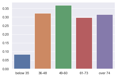
Age: People below age 35 as a group were little interested in getting a Credit card whereas people from age group 36 to 60 were the most interested ones.
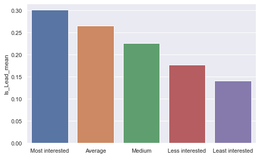
Region code: I grouped certain regions into groups according to their interest in getting a Credit card. Out of which RG283, RG284, RG268 were the regions from which we got the people who are most likely to get a Credit card.
Occupation: Customers who earn with Salaried based jobs are the ones who would be less likely to get a Credit card whereas Entrepreneurs are most likely to get a Credit card and that too with a large margin as compared to other occupations.
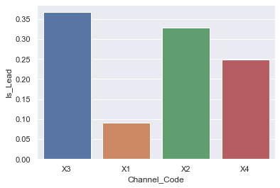
Channel Code: Customer caring from X3 and X2 acquisition channe;s are more likely to get a Credit card.
Vintage: The bank has a lot of customers who have joined recently in around 20 months, but they are not the ones who are showing interest in getting a Credit card. It is about trust with the bank and we observe that the customers who have been customers since 85 to 109 months are the ones who are more likely to get the Credit card.
Credit Product: If someone already has an active credit product i.e. any kind of loan they are more likely to get the Credit card.
Occupation and Credit product: Entrepreneurs don't seem to have any active credit product.
Average account balance: Customers who are interested in getting a Credit card are the ones who have a larger Average account balance which is above $110000.
Is_active: If a customer is active for a minimum of 3 months then he/she is more likely to get a Credit card.


Feature engineering:
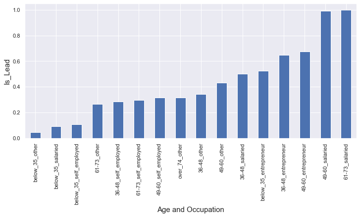
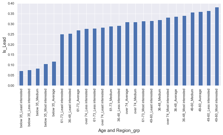
I created 3 new features where I combined ‘Age’ with ‘Region code’, ‘Occupation’ and ‘Channel code’ such that you’ll get people with different age groups grouped with their Occupation, Region code and Channel code. And now we can see which combination is showing the most interest.
age_occ: All Entrepreneurs below age 60 and Salaried people from age 49 to 73 are more likely to show interest. And the ones who are least interested are everyone below age 35 except Entrepreneurs.
age_chan: Customers coming from X1 acquisition and are below age 48 and the customers coming from X3 acquisition and are below age 35 are least likely to get a Credit card. But if a customer is coming from X3 and is of the age group 36 to 60 is the one who is more likely to get a Credit card.
age_reg: If a customer is below age 35 it doesn't matter which region he/she belongs to, they’ll show the least interest. On the other hand if a customer is from age group 49 to 60 it is going to show interest except he/she is from the ‘Least interested’ region group.

Preprocessing before model building:
I encoded categorical data with .map() and LabelEncoder methods. I also took the square root of feature ‘Average account balance’ so that the magnitude of elements of the feature could be decreased, so that the difference between scales of feature doesn't mess with training of model and model can treat every feature equally while training. Now the data was ready to get divided into Input and Output data. After dividing the data I used the train_test_split() method to split the data into training and test data with 80-20 split respectively for the model to get trained and tested on.
Model building:
For modeling, I initially imported Logistic regression, Decision tree classifier and Random forest classifier models since this is a classification problem and trained these models over the trained data and checked the accuracy of all the models. Accuracies that I found were not that good, so I removed all the feature engineering where I had grouped and then encoded the data and then trained the models again with a new train and test split and found the accuracy has increased a lot. New accuracies were around 84.65% to 85.70%. Now to see if I can get accuracy by trying better models, I learned Boosting models.
Boosting:
To describe in short, Boosting and Bagging are 2 different types of Ensemble learning which is a method that is used to enhance the performance of machine learning models by combining several learners. This type of learners build models which improve efficiency and accuracy. The Decision tree and Random forest belong to the Bagging type. Principle behind bagging is dividing your dataset into different bootstrap dataset and you are running an algorithm on each of these data sets parallely. Boosting is basically doing this but sequentially instead of parallely that too with updating the weights depending on misclassified samples in previous bootstrapped data.
There are 3 different types of Boosting primarily:
(1) Adaptive boosting.
(2) Gradient boosting.
(3) XG boost(Extreme gradient boosting).
Adaptive boosting: In adaptive boosting these are the steps the model follows:
Step 1: Initially each observation is weighed equally for the first decision stump.
Step 2: After the training misclassified observations are assigned higher weights.
Step 3: Then a new decision stump is drawn by considering the observations with higher weights as more significant .
Step 4: Again if any observations are misclassified, they are given higher weight.
Step 5: The process continues until all the observations fall in the right class.
Python code to implement this model is given below.
Gradient boosting: In gradient boosting, base learners are generated sequentially in such a way that the present base learner is always more effective than the previous one. Overall model improves sequentially with each iteration. Only difference is that it does not increment the weight of misclassified observations. It actually optimizes the loss function of the previous learner by adding a new adaptive model that adds a weak learner in order to reduce the loss function. Main idea here is to overcome the errors of previous predictions. Python code to implement this model is given below.
XG boost: XG boost is basically an advanced version of Gradient boosting method that is designed to focus on computational speed and model efficiency. In order to do this it has a couple of features. It supports parallelization by creating decision trees parallely. It uses the Distributed Computing method for evaluating only large and any complex methods. It also uses core computing in order to analyze huge and varied datasets. It implements cache optimization in order to make best use of your hardware and all your resources overall. Python code to implement this model is given below.
There are also other boosting models like Light gbm (Light gradient boost machine) and Cat boost(Category boost).
Light gbm: It is a fast, distributed high performance gradient boosting framework based on the decision tree algorithm. Lgbm splits the tree leaf wise with the best fit whereas other boosting algorithms split the tree depth wise or level wise. This leaf wise algorithm can reduce more loss function than the level wise algorithm hence results in better accuracy. It is surprisingly very fast hence the word ‘Light’. Python code to implement this model is given below.
Cat boost: It is a high-performance open source library for gradient boosting on decision trees. It reduces time spent on parameters tuning because it provides results with default params. It allows you to use non-numeric factors, you don't have to turn categorical data into numeric data. It is fast because it uses a multi configuration for large datasets. It also reduces overfitting when constructing your model with a novel gradient boosting scheme.
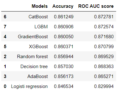
So I tried all of these models and found the better accuracy according to the better ROC-AUC score since that was the criterion for this project. I created a DataFrame with model name, accuracy and ROC-AUC score and sorted descendingly to ROC-AUC score. Cat boost and Lgbm were giving very close accuracy and ROC-AUC score and were followed by Gradient boosting and XG boost.


Feature selection:
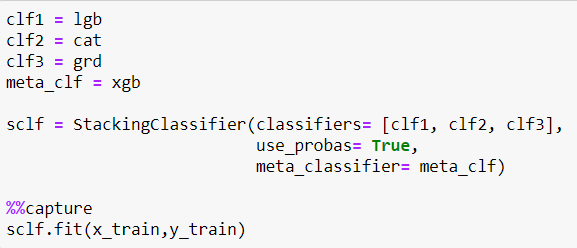
Since Lgbm and Cat boost were too close in competition I was advised to try Stacking classifier with Lgbm, Cat boost and Gradient boost being the 3 base models and XG boost being the meta model. What Stacking classifier does is it further splits train data into other train data and validation data. Then trains base models on train data and uses its prediction probabilities to meta model and validate on validation data. Which collectively gives better and non-overfitting models. But the accuracy and ROC-AUC score which I got was lesser than Catboost so I decided to stick with the Catboost model.
After deciding Catboost models as the final model, only one last step is remaining, that is feature selection on feature importance. With using ‘cat.feature_importance_’ I listed out features on the basis of how important they are for predicting the target variable and started dropping one feature at a time with the least feature importance value and checked the accuracy of each new Catboost model and stopped when the accuracy of the new Catboost model started decreasing as compared to the initial Catboost model. This resulted in a little bit increase in accuracy if I dropped the feature ‘Gender’ and that's how I settled on the new Catboost model and used that model to predict Lead generation on the main Test data.
Conclusion:
In this project I got to learn about new models and Stacking and Blending methods. So even though I couldn't be on the leaderboard of the competition in the end, doing this project added a lot to my skill set and knowledge. All thanks to my mentor Mr. Shyambhu Mukherjee who helped me through this project.
Comments
Post a Comment