Exploring the Automl and pandas profiling using titanic dataset

        Exploring automl and pandas profiling using titanic dataset

                              project and writing: shyambhu mukherjee

Introduction:

In this project, we created a kaggle notebook on the titanic dataset and explored two new items:

(1) sberbank light automl library

(2) pandas profiling

In this blog post, I am going to describe the project; different code patches and how the whole thing worked out.

Pandas profiling to start:

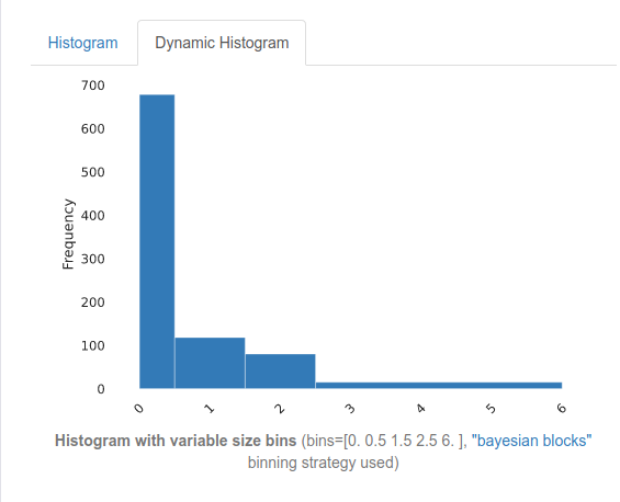
If you don't know what is pandas profiling, then let me introduce to it. Basically pandas dataframe has a describe attribute; which let's you see the count,mean, median, 75%, and max of the columns in the dataframe. The pandas profiling is an extended version of that; which sort of automates the whole task of exploring and creating a large number of eda outputs. 

In short, here are the things which pandas profiling does:

(1) create basic statistics of the variable with mentioning how many are unique, what is the count, if there are any missing values or not and so on so.

 (2) provide common, extreme minimum and extreme maximum values.

(3) Create both basic and dynamic histograms with advanced binning strategies.

(4) provide correlation charts with 5 different types of correlation; i.e. pearson'r , spearman's rho, kendall's to, phik, cramer's v. 

(5) Lastly it also provides missing values for each columns, sample first 5 values, last 5 values.

 

As you can see therefore, pandas profiling gives you immense number of exploratory data analysis output within minutes; and the quality and number of explorations are enough for a small data like this also to go through and create different insights, understanding and all. 

We went through this eda and came up with the following insights:

1. from correlation matrix, it can be seen that passenger class i.e. pclass is a strong indicator of the fact that belonging to 3rd or 2nd classes represented lower survival rates which is true from historical anecdotes.
   
2. age is also a slight negative marker of survival. Being higher age is slightly negatively correlated with survival so representing lesser survival with increasing age.
   
3. Fare is again a strong indicator of survival; i.e. increasing fair has medium amount of correlation with survival.
   
4. Fare was not positive with every case. 15 people rode the ship with 0 fare. That maybe due to special treatment or people free- riding the ship. We can create a feature Is_fare_0 to check how that relates with survival.
   
5. Some people paid pretty high fares. I wonder how they were treated. We will create a feature called VIP_fare for people who paid more than 112.07915; the 95th percentile.
   
6. I think extreme ages are also concernable. Historic anecdotes say that there have been preferences to women and children. Creating a feature age_less_10 which denotes if age is less than 10; makes sense. Age is missing in some cases. I wonder what leads to that. We will create a feature if_age_missing and put 0 if age is present and 1 if age is missing.
   
7. parch and sibsp are interesting features too. parch refers to number of parents / children aboard the Titanic.
   
8. Cabin is not present for many passengers. Cabin is for sure a signal of lavishness therefore. We will check if having cabin is a signal for survival.
   Let's create the features and run one round of automl on the features.

From this, we generated these features and prepared the dataset. The training dataset also had two missing elements as pointed out by pandas profiling earlier; which we filled by the median value.

After this, we implemented the automl library and tried out the full pipeline. The sberbank automl is a pipeline based automl library; which let's you put each of the components into its automl pipeline. 

But as you will see; the automl is not that good. The few downpoints I pointed out from the example notebook code which I thoroughly followed is that there is just too much code we need to write even though it is automl. Many automl features instant coding and 2-lines of code lead to immense calculation and poof! out comes the model. But not here.

In sberbank automl, you have to specifically write out the automl components, provide parameters even and then finally add the model up with pipelines and create the automl. Only thing which happens automatic thereafter is that it runs a number of different hyperparameters; and xgboost and lightgbm models inside the pipeline and gives out a automl model which it considers to be the best in performance.

While that is what is claimed, sad thing is that the automl generated model generated only 0.77 score in the titanic leaderboard. In turn a small 100 tree and 4 layer deep random forest created and fine tuned manually by me generated 0.78 score; and ranked me in top 20%. 

So I am not sure that I would recommend the lightautoml model to use. But what I will still do is; provide you the link of the code. Before that, do watch this video to provide a good word about the light automl model from the writers.

Also, one of the main things which LAMA focuses on is the time of training. Upon completing the automl calculation; LAMA gives you a html report; where you can find out time spent total to train the model and where are the bottlenecks and issues in probably training the model. This is a cool feature to use LAMA for. 

My view here is not to be taken as a permanent measure as my data is extremely small; a category where LAMA is supposedly not that great from other automls as well as I am still learning about LAMA as well as LAMA is itself getting worked upon actively. So while I will not recommend it to replace any automl you are using and have tested performances; I do appreciate you to use and explore it.

Here are the code snippets of what I did with LAMA. I followed this notebook from examples and implemented the code on my data as it is. For using a preset automl pipeline, you have to follow this notebook.

So as I was discussing, there are 4 steps if you create the pipeline from your end. Even on preset, you have to go through most of these steps; therefore I chose to take the slightly longer path anyway.

First step is to import the components and setting your data. This is how we did that.

from lightautoml.automl.base import AutoML
from lightautoml.ml_algo.boost_lgbm import BoostLGBM
from lightautoml.ml_algo.tuning.optuna import OptunaTuner
from lightautoml.pipelines.features.lgb_pipeline import LGBSimpleFeatures
from lightautoml.pipelines.ml.base import MLPipeline
from lightautoml.pipelines.selection.importance_based import ImportanceCutoffSelector, ModelBasedImportanceEstimator
from lightautoml.reader.base import PandasToPandasReader
from lightautoml.tasks import Task
from lightautoml.utils.profiler import Profiler
from lightautoml.automl.blend import WeightedBlender

import logging
import os
import time
logging.basicConfig(format='[%(asctime)s] (%(levelname)s): %(message)s', level=logging.INFO)

# Installed libraries
from sklearn.metrics import roc_auc_score
from sklearn.model_selection import train_test_split
import torch

N_THREADS = 8 # threads cnt for lgbm and linear models
N_FOLDS = 5 # folds cnt for AutoML
RANDOM_STATE = 42 # fixed random state for various reasons
TEST_SIZE = 0.1 # Test size for metric check

np.random.seed(RANDOM_STATE)
torch.set_num_threads(N_THREADS)

p = Profiler()
p.change_deco_settings({'enabled': True})

TARGET_NAME = 'Survived'# target column name

train_main_data, test_main_data = train_test_split(train_data_mod, 
                                                   test_size=TEST_SIZE, 
                                                   stratify=train_data[TARGET_NAME], 
                                                   random_state=RANDOM_STATE)
logging.info('Data splitted. Parts sizes: train_data = {}, test_data = {}'
              .format(train_main_data.shape, test_main_data.shape))

%%time

task = Task('binary')
reader = PandasToPandasReader(task, cv=N_FOLDS, random_state=RANDOM_STATE)    

The second step is to create feature selector. We basically achieved that by creating light gbm and letting the feature importance from that to choose the best features. Now, I don't know much about lgbm; but as that is not a uniquely better algorithm; therefore this may serve as a bottleneck for the performance of the automl model as it depends on that.

%%time

model0 = BoostLGBM(
    default_params={'learning_rate': 0.05, 'num_leaves': 64, 'seed': 42, 'num_threads': N_THREADS}
)
pipe0 = LGBSimpleFeatures()
mbie = ModelBasedImportanceEstimator()
selector = ImportanceCutoffSelector(pipe0, model0, mbie, cutoff=0)

Output: 

Copying TaskTimer may affect the parent PipelineTimer, so copy will create new unlimited TaskTimer

CPU times: user 2.89 ms, sys: 1.01 ms, total: 3.89 ms
Wall time: 3.62 ms

#check the time; it's very low even for 800 row dataset. This is a good point for big data.

In the third step, we create the pipeline. We actually create two layers for the pipeline and then add them together to create the pipe. Here's how exactly we achieve that:

Step 3.1. Create 1st level ML pipeline for AutoML

Our first level ML pipeline:

• Simple features for gradient boosting built on selected features (using step 2)
• different models:
  • LightGBM with params tuning (using OptunaTuner)
  • LightGBM with heuristic params

 

%%time 

pipe = LGBSimpleFeatures()

params_tuner1 = OptunaTuner(n_trials=20, timeout=30) # stop after 20 iterations or after 30 seconds 
model1 = BoostLGBM(
    default_params={'learning_rate': 0.05, 'num_leaves': 128, 'seed': 1, 'num_threads': N_THREADS}
)
model2 = BoostLGBM(
    default_params={'learning_rate': 0.025, 'num_leaves': 64, 'seed': 2, 'num_threads': N_THREADS}
) 

Step 3.2. Create 2nd level ML pipeline for AutoML

Our second level ML pipeline:

• Using simple features as well, but now it will be Out-Of-Fold (OOF) predictions of algos from 1st level
• Only one LGBM model without params tuning
• Without feature selection on this stage because we want to use all OOFs here

pipeline_lvl1 = MLPipeline([
    (model1, params_tuner1),
    model2
], pre_selection=selector, features_pipeline=pipe, post_selection=None)

%%time

pipe1 = LGBSimpleFeatures()

model = BoostLGBM(
    default_params={'learning_rate': 0.05, 'num_leaves': 64, 'max_bin': 1024, 'seed': 3, 'num_threads': N_THREADS},
    freeze_defaults=True
)

pipeline_lvl2 = MLPipeline([model], pre_selection=None, features_pipeline=pipe1, post_selection=None) 

output: CPU times: user 1.18 ms, sys: 14 µs, total: 1.19 ms
Wall time: 1.2 ms  

Now, after this, it is just calling the automl model and fitting it. 

Step 4. Create AutoML pipeline

AutoML pipeline consist of:

• Reader for data preparation
• First level ML pipeline (as built in step 3.1)
• Second level ML pipeline (as built in step 3.2)
• Skip_conn = False equals here "not to use initial features on the second level pipeline

 

%%time 

automl = AutoML(reader, [
    [pipeline_lvl1],
    [pipeline_lvl2],
], skip_conn=False)

Step 5. Train AutoML on loaded data

In cell below we train AutoML with target column TARGET to receive fitted model and OOF predictions:

%%time 

oof_pred = automl.fit_predict(train_main_data, roles={'target': TARGET_NAME})
logging.info('oof_pred:\n{}\nShape = {}'.format(oof_pred, oof_pred.shape))  

So this is where the actual fitting happens. This outputs a long copy of model training results with roc-auc validation scores; early stopping outputs and all. A good improvement will be to actually provide this as a report too. And I recently filed a issue in the repo for the same. 

After this step, we can analyze the feature selection and the different performance criteria of the automl.

Step 6. Analyze fitted model

Below we analyze feature importances of different algos:

logging.info('Feature importances of selector:\n{}'
              .format(selector.get_features_score()))
logging.info('=' * 70)

logging.info('Feature importances of top level algorithm:\n{}'
              .format(automl.levels[-1][0].ml_algos[0].get_features_score()))
logging.info('=' * 70)

logging.info('Feature importances of lowest level algorithm - model 0:\n{}'
              .format(automl.levels[0][0].ml_algos[0].get_features_score()))
logging.info('=' * 70)

logging.info('Feature importances of lowest level algorithm - model 1:\n{}'
              .format(automl.levels[0][0].ml_algos[1].get_features_score()))
logging.info('=' * 70) 

Step 7. Predict to test data and check scores

%%time

test_pred = automl.predict(test_main_data)
logging.info('Prediction for test data:\n{}\nShape = {}'
              .format(test_pred, test_pred.shape))

logging.info('Check scores...')
logging.info('OOF score: {}'.format(roc_auc_score(train_main_data[TARGET_NAME].values, oof_pred.data[:, 0])))
logging.info('TEST score: {}'.format(roc_auc_score(test_main_data[TARGET_NAME].values, test_pred.data[:, 0])))

Step 8. Profiling AutoML

To build report here, we have turned on decorators before during initialization of variables. Report is interactive and you can go as deep into functions call stack as you want:

%%time
p.profile('my_report_profile.html')
assert os.path.exists('my_report_profile.html'), 'Profile report failed to build' 

Here's how the report looks like.

The arrows open up to each details and logs the amount and percentage of time that process takes. This is a thing which is pretty useful. 

So this ends our exploration of automl and pandas profiling. While my first experience with this library was not the best with the low score; as the creators suggest; I will however use it with bigger dataset and update y'all about the time advantages and performance of the models. One more aspect to try out with this model is to check if and how does it train automatic neural network models. 

So thanks for reading this article. We created some more variables and actually achieved the top 18% rank with a small random forest model. But that is a tale for another day. For now, stay tuned and happy reading!